Archive for category OpenCv

Cartesio – low cost cartesian plotter robot


Recently the famous site evilmadscientist introduced the new art robot called “Axidraw“.I saw the robot in action and it is very similar to the robot I built in the 2015, called “Cartesio”, a 3d printed cartesian robot.  So, I decided to publish  in open source all the details about Cartesio.


Cartesio is similar to Axidraw, the main differences are:

– Cartesio is a cartesian robot (xy movement) while Axidraw is a type of corexy movement (t-bot I think)

– Cartesio is based on Arduino, while Axidraw is based on the EBB Driver board

– Cartesio has a large working area (40×30), like an A3 paper, while Axidraw has a normal working area (30×20), like an A4 paper.

– Cartesio is 3d printed, while Axidraw is in metal (? this is not very clear watching the pictures)

– Axidraw can write with a fountain pen, Cartesio not (yet)

– Axidraw costs 450$, Cartesio costs 60$. Not bad!


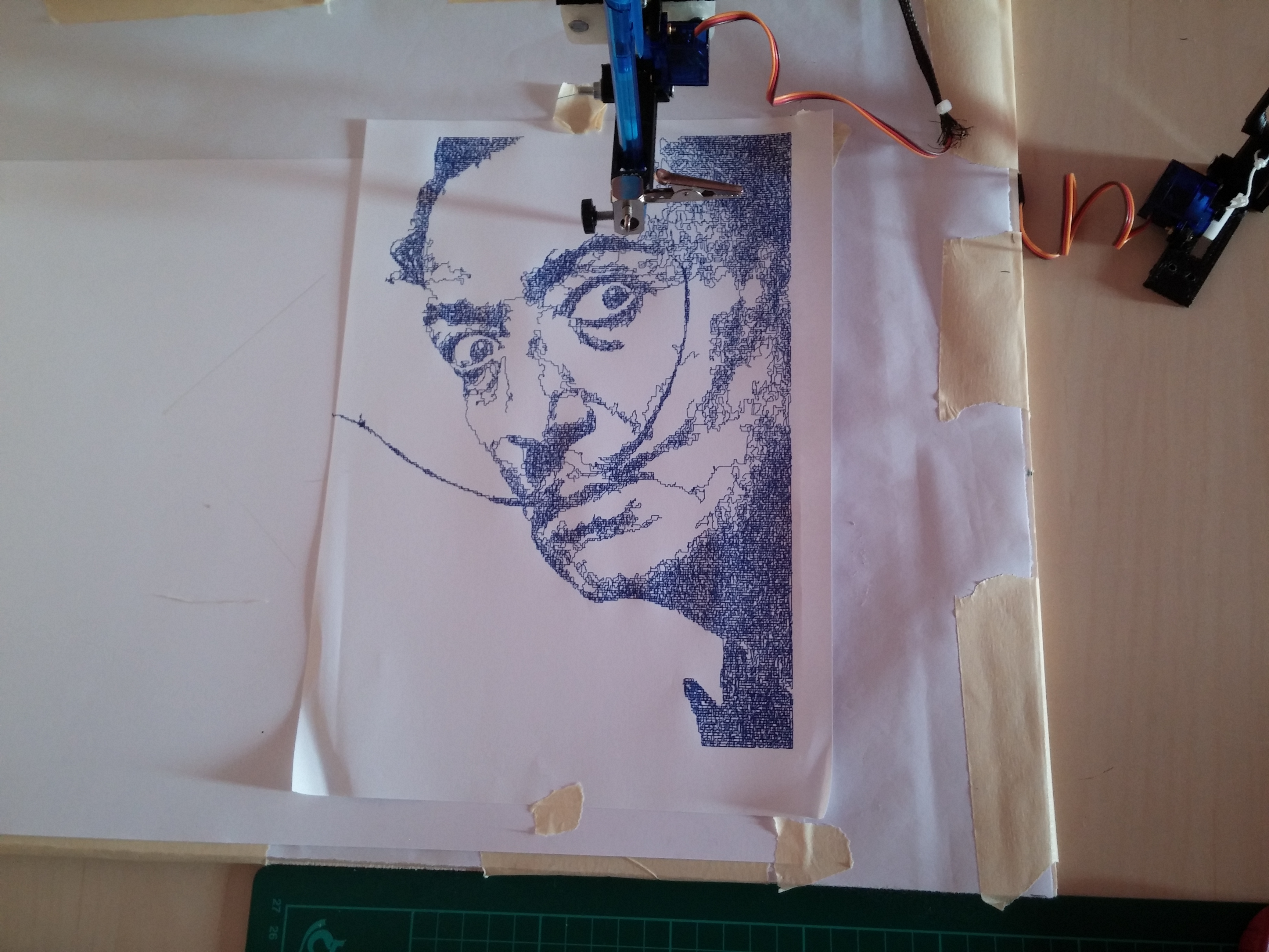
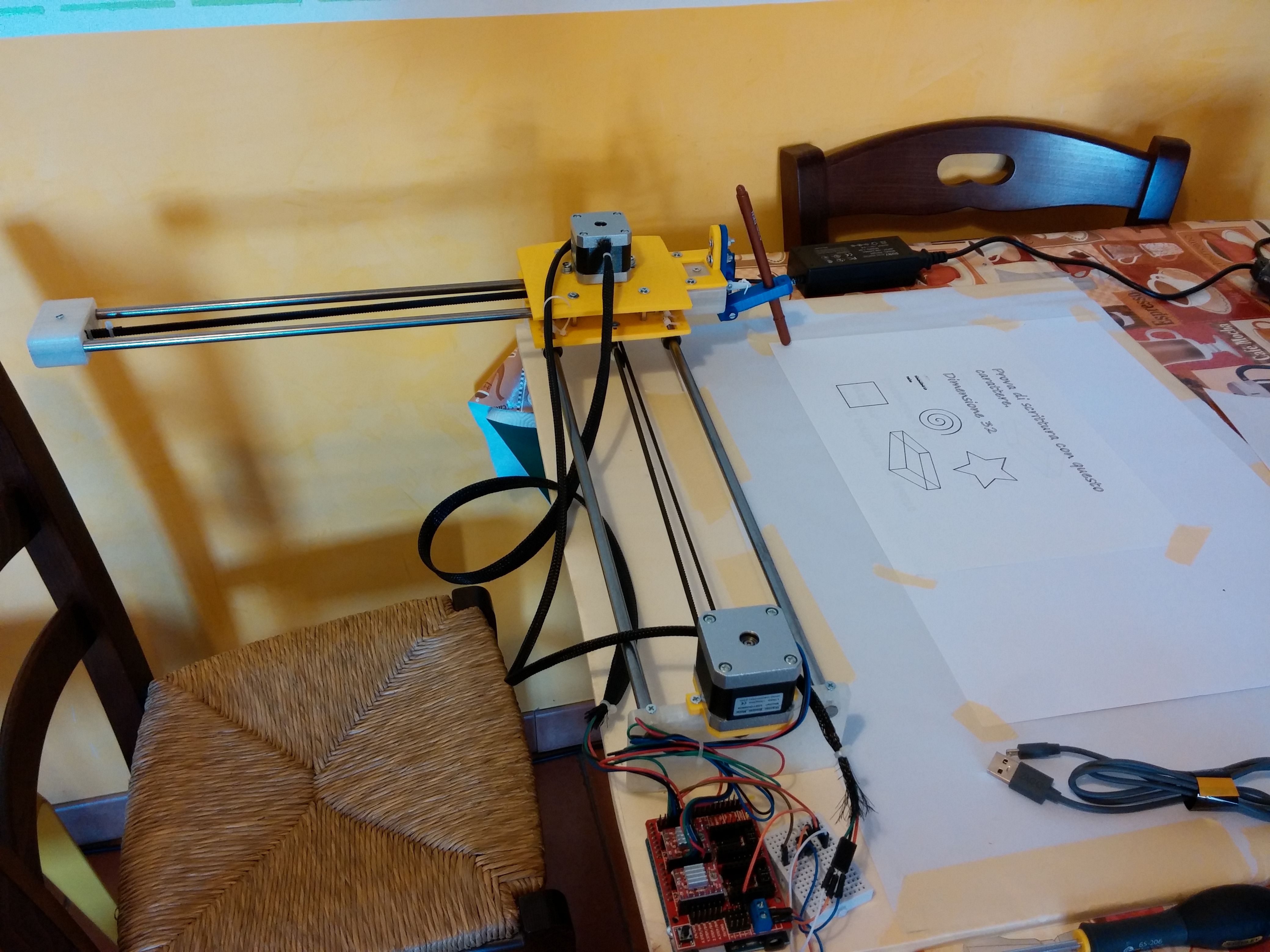
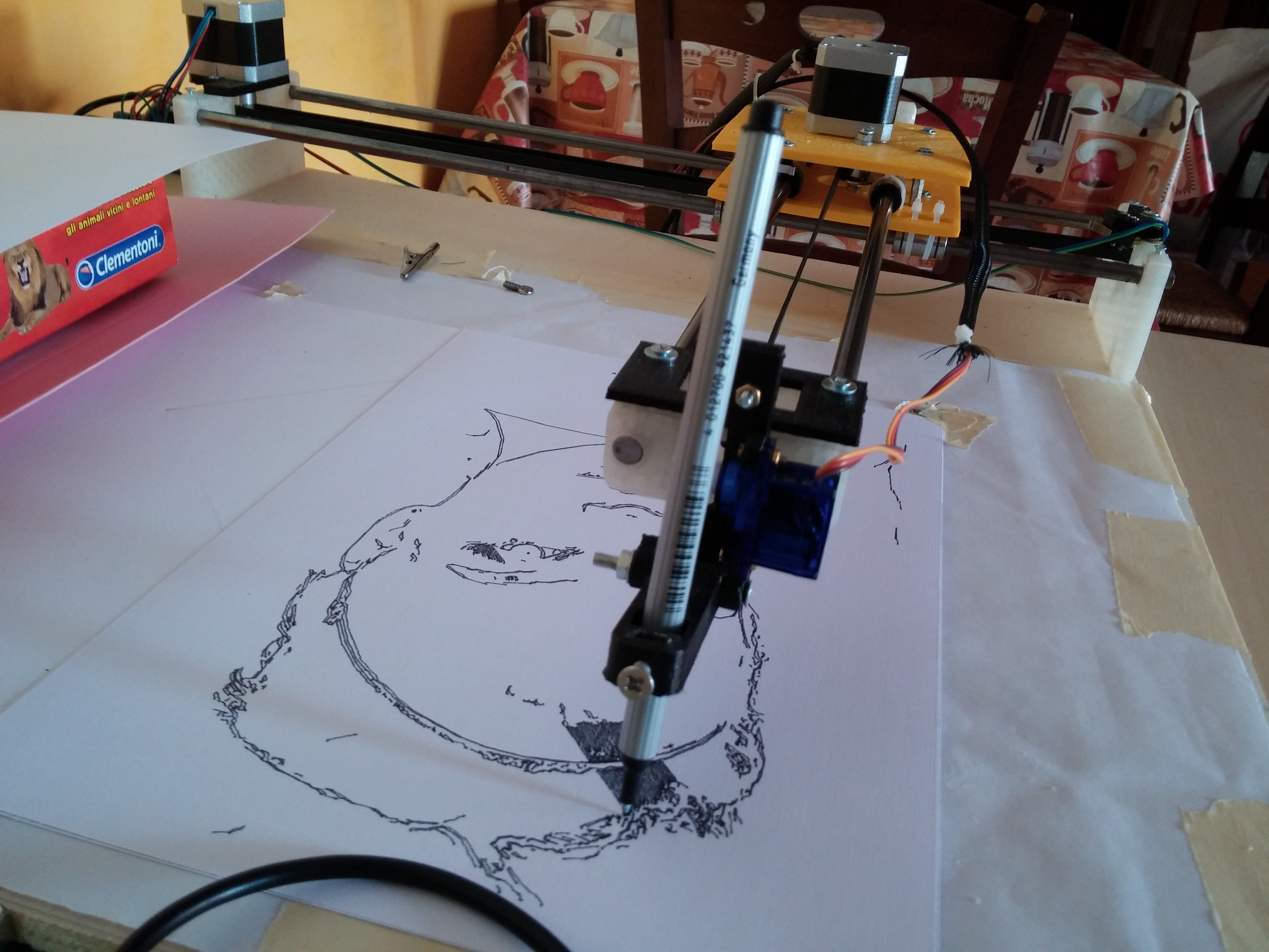
I’m interested in robots that can draw so in the last years I made many drawing robots. Cartesio is the last experiment. I saw a cartesian arm and it was very interesting, so I decided to build one.  Here you can see the robot in action:


Here some drawings made with Cartesio.

 20150623_075035DSCF206420150716_204807 20150715_22444520150716_06493020150717_20263620150717_202652


20150708_200255DSCF2066DSCF2043


DSCF2057


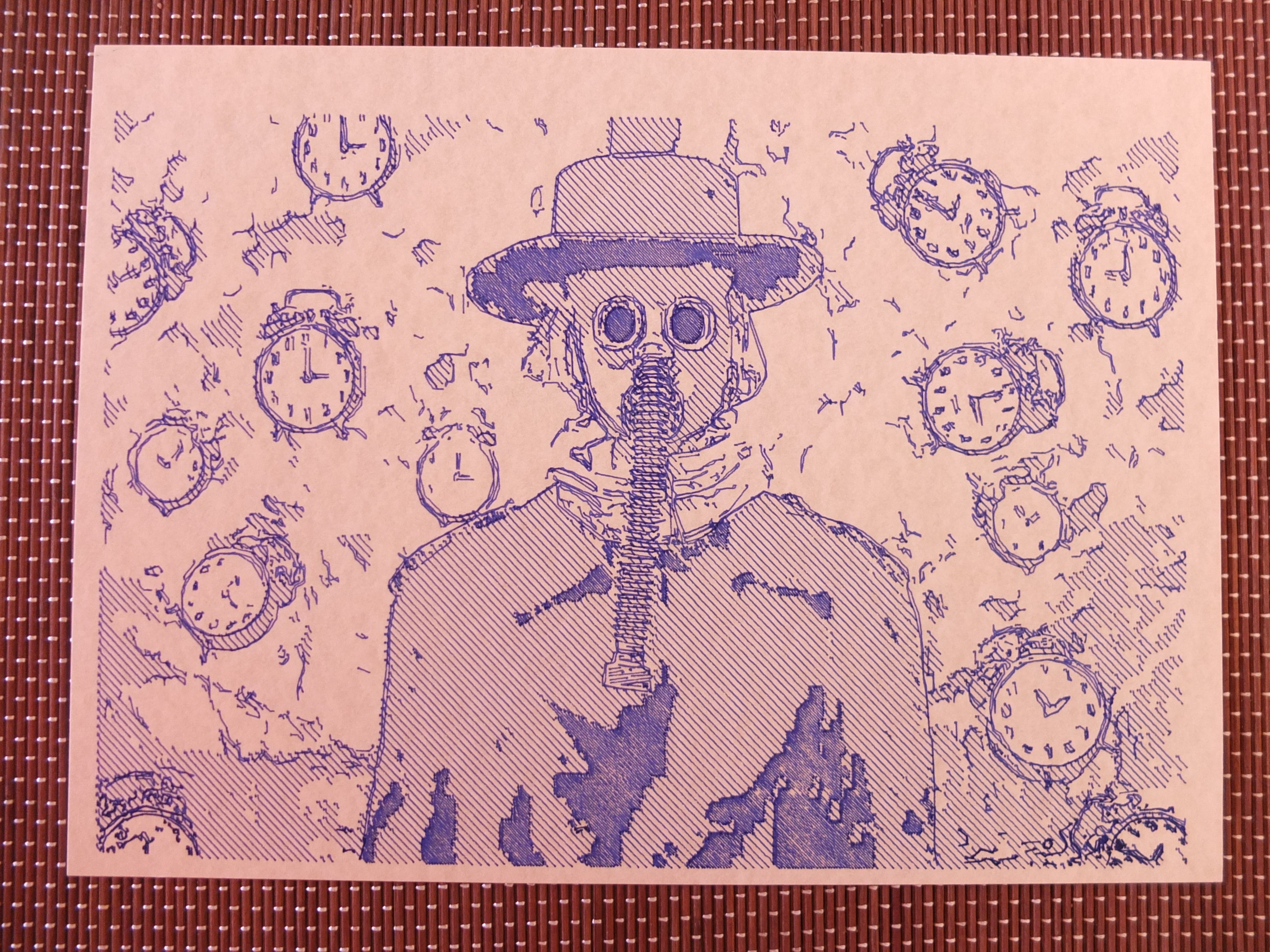
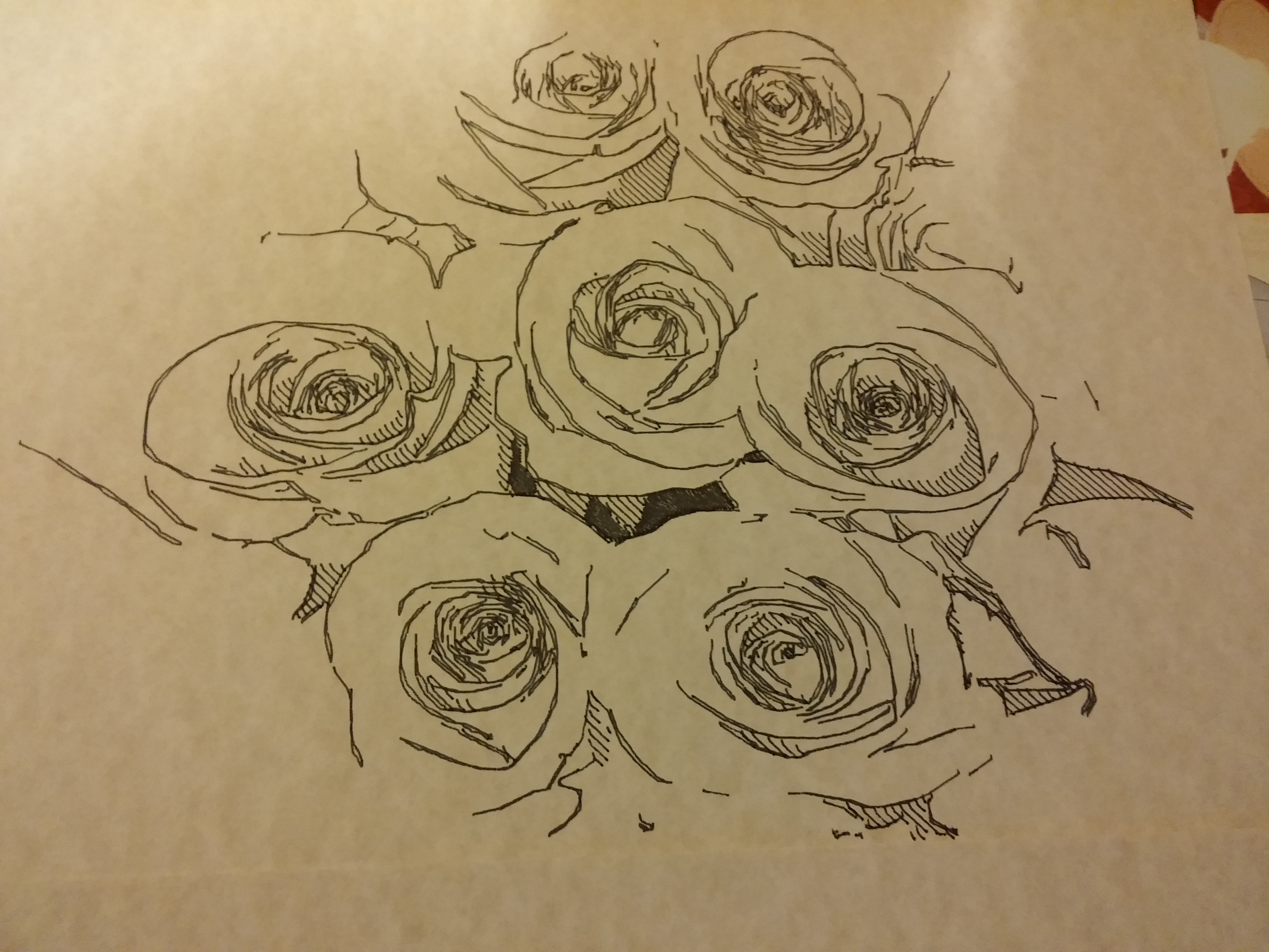
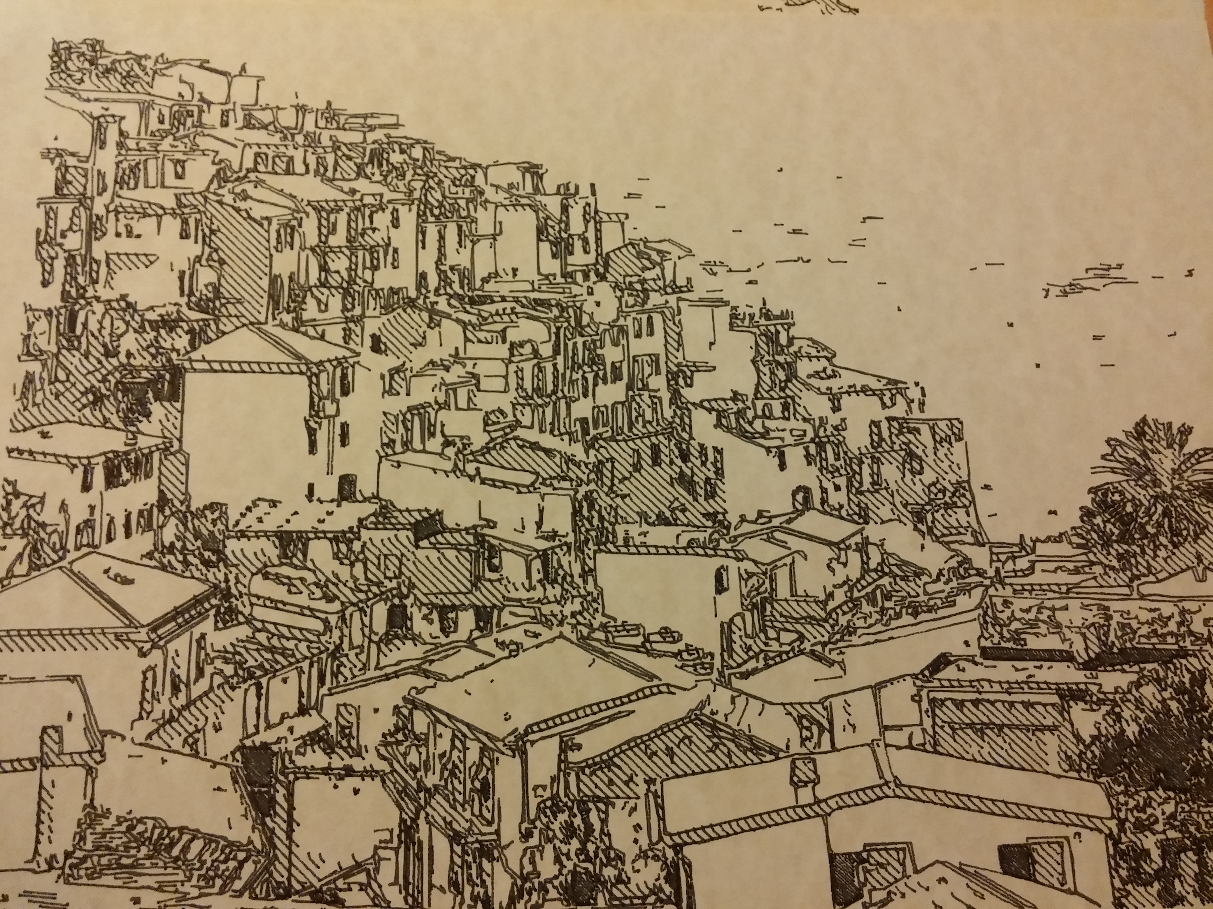
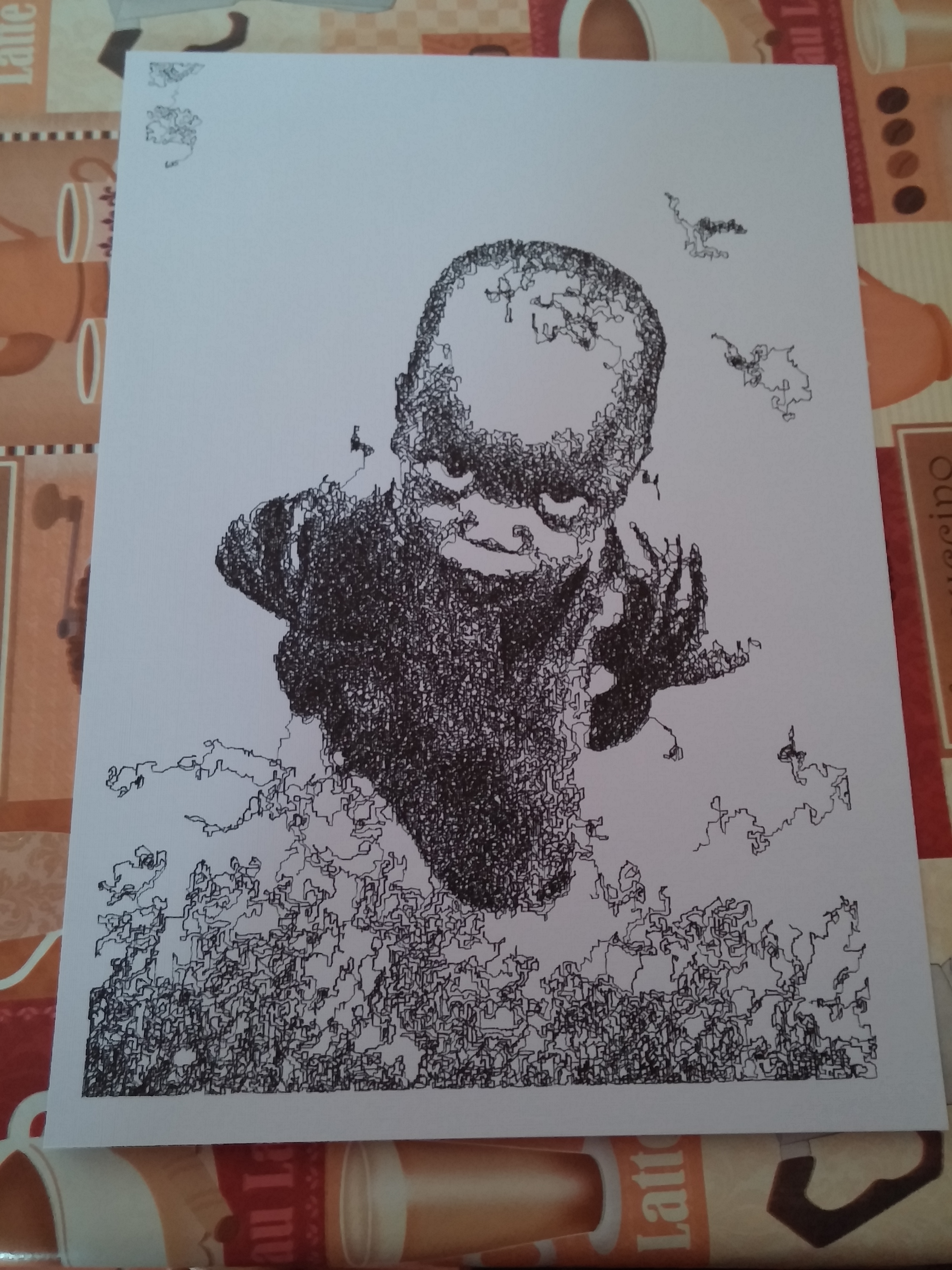
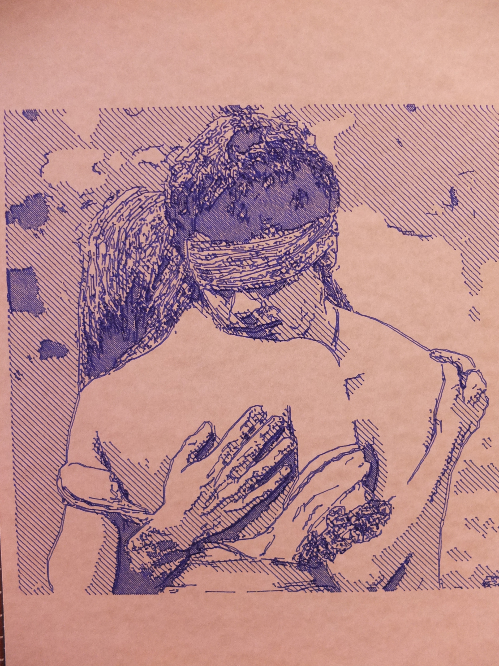
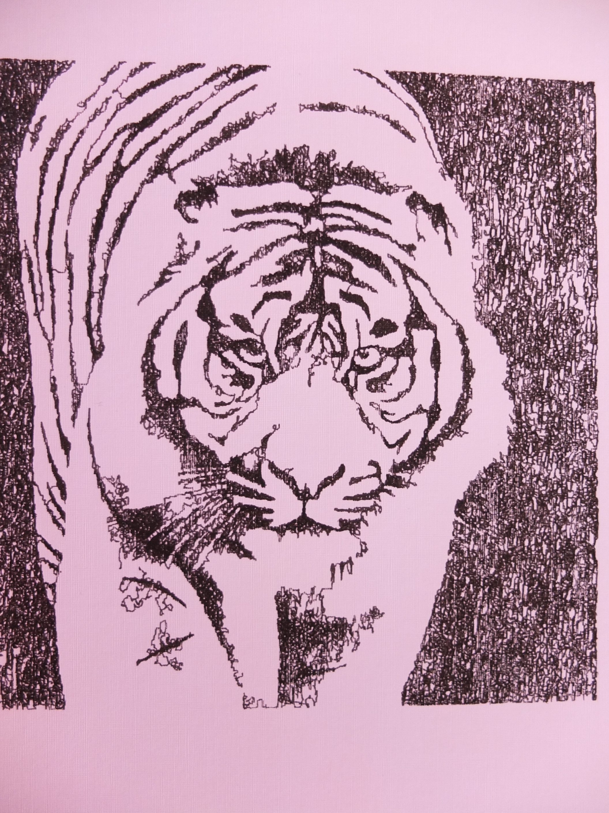
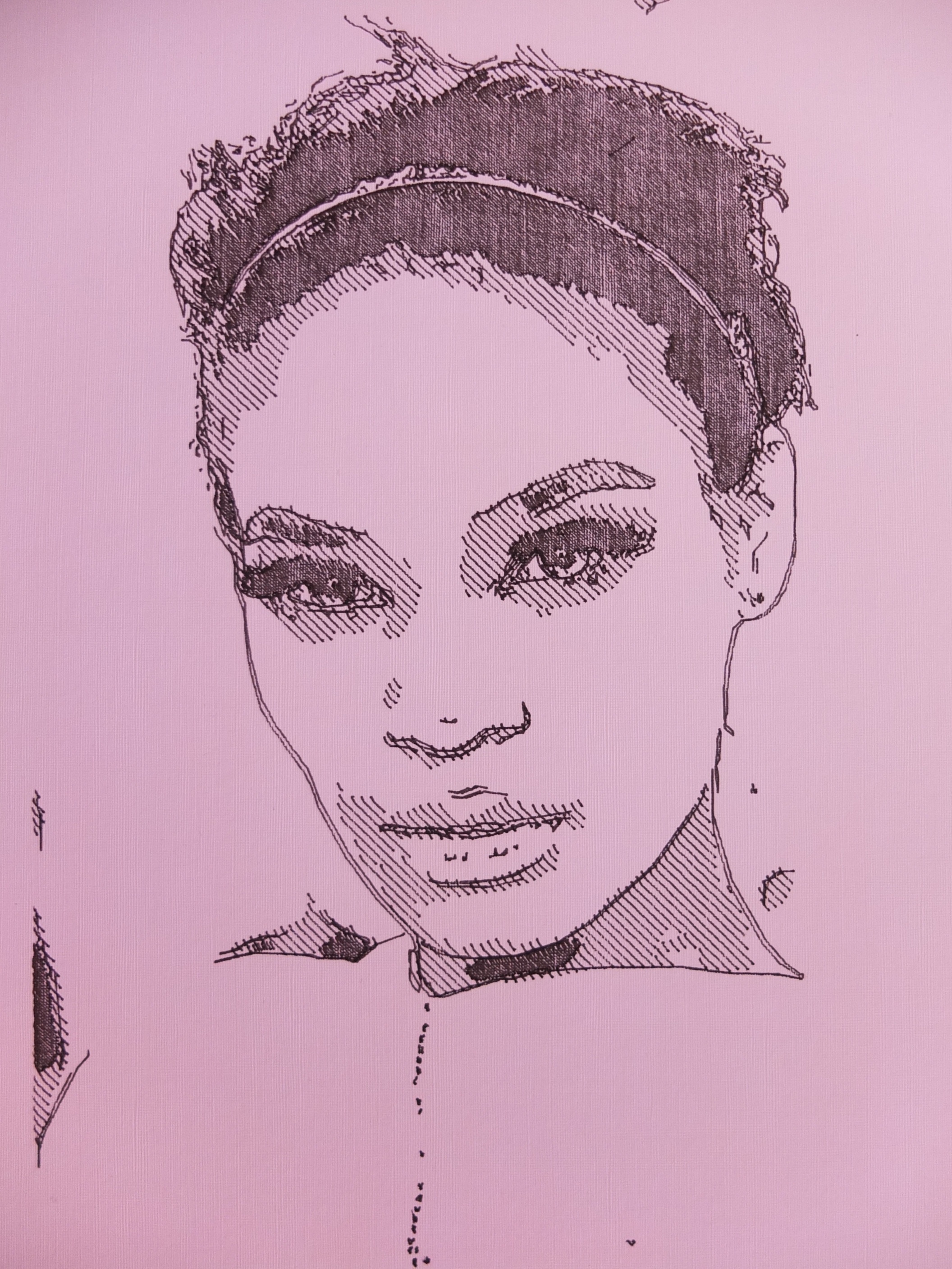
You can find more pictures here.


Hardware:

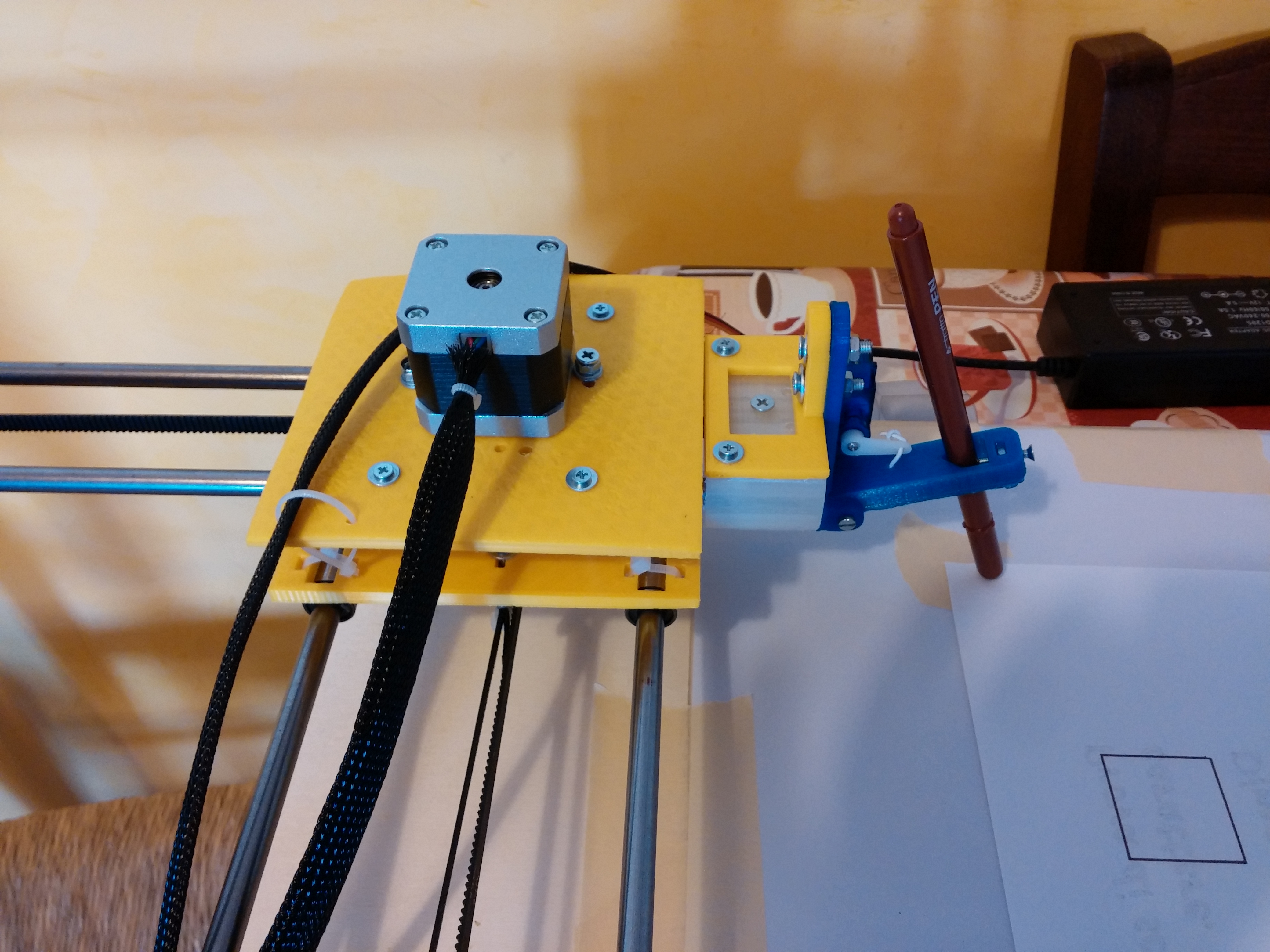
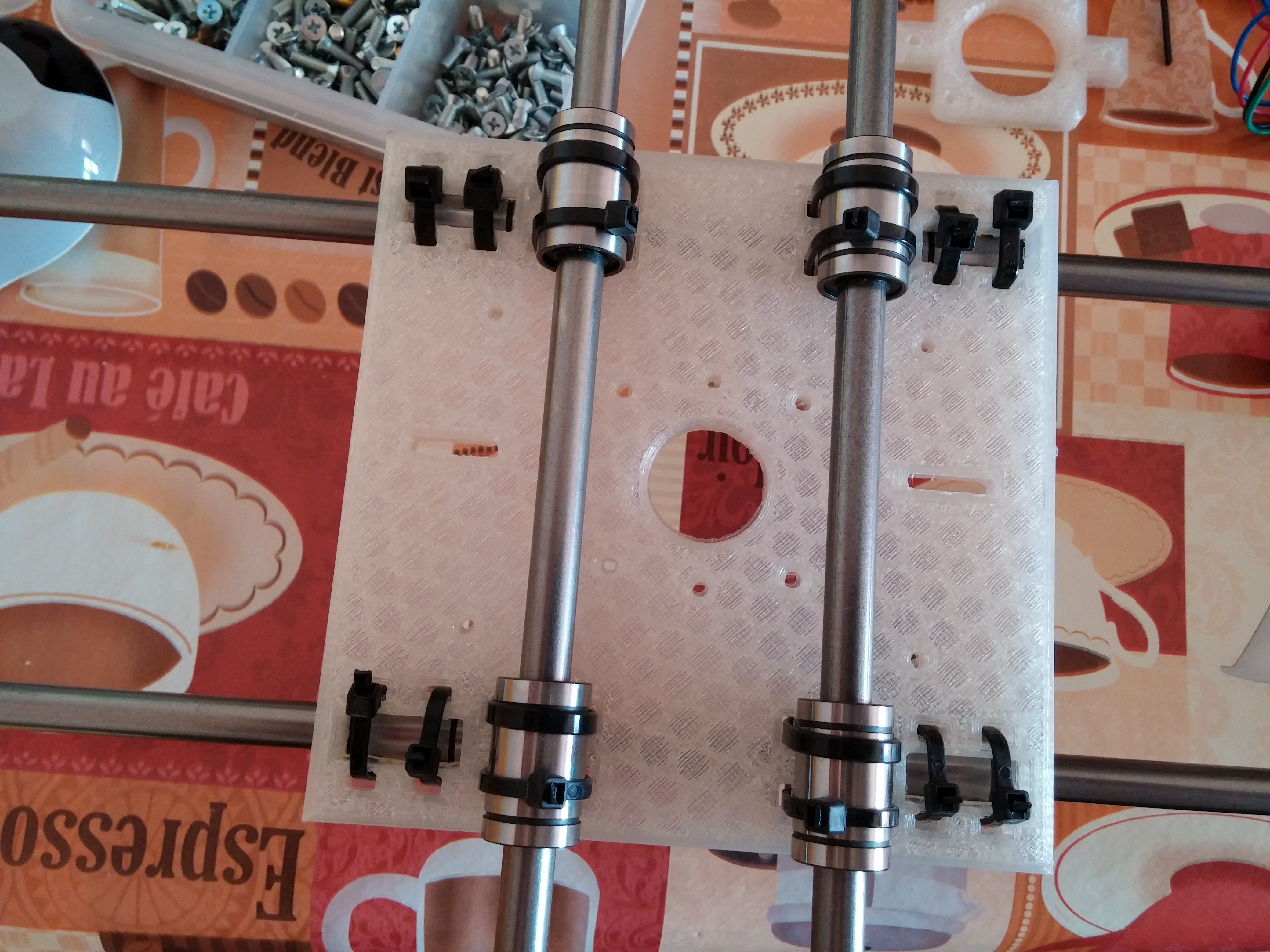
Cartesio is built using M8 smooth rods and LM8UU bearings, GT2 belt, some printed plastics. Standard components, easy to find.


PLASTICS

All the plastics are made with a standard 3d printer (in PLA). You can find the files to print the plastics here.


BOM HW:

– 4x smooth rod M8 – 500 mm – Link

– 4x bearing 624zz – Link

– 8x bearing LM8UU  – Link

– 1000 mm GT2 belt – Link

– 2x GT2 Pulley – Link

– 4x M3 spacers 30mm

– M3 and M4 screws and nuts

– some plastic cable ties

– a pen


BOM Electronics:

– Arduino Uno

– Arduino CNC shield – Link

– 2x  A4988 driver

– 2 stepper motor Nema17 + wires

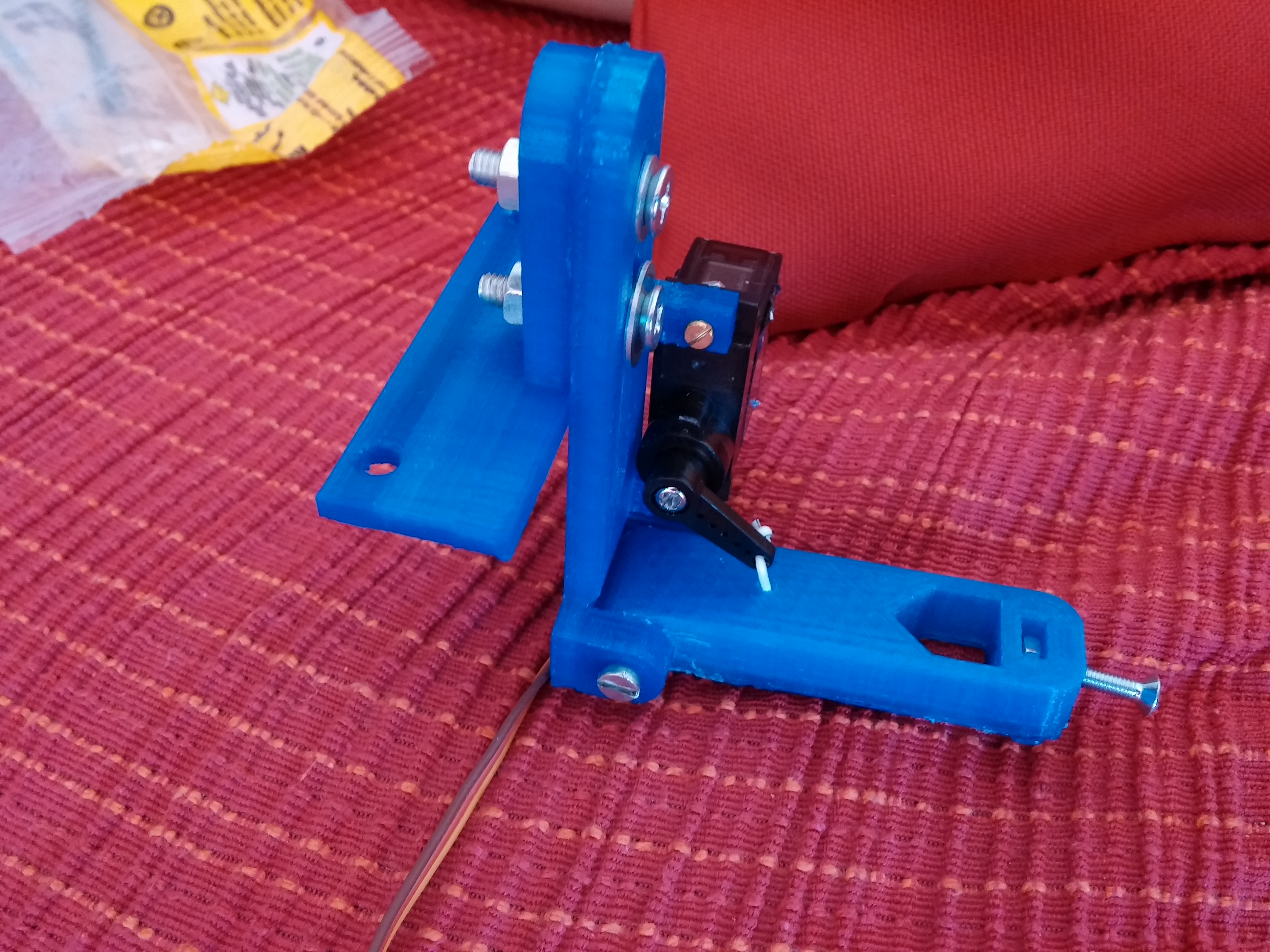
– 1 servo 9g + wires

– 2 mechanical endstop + wires

– 12v 5A power supply
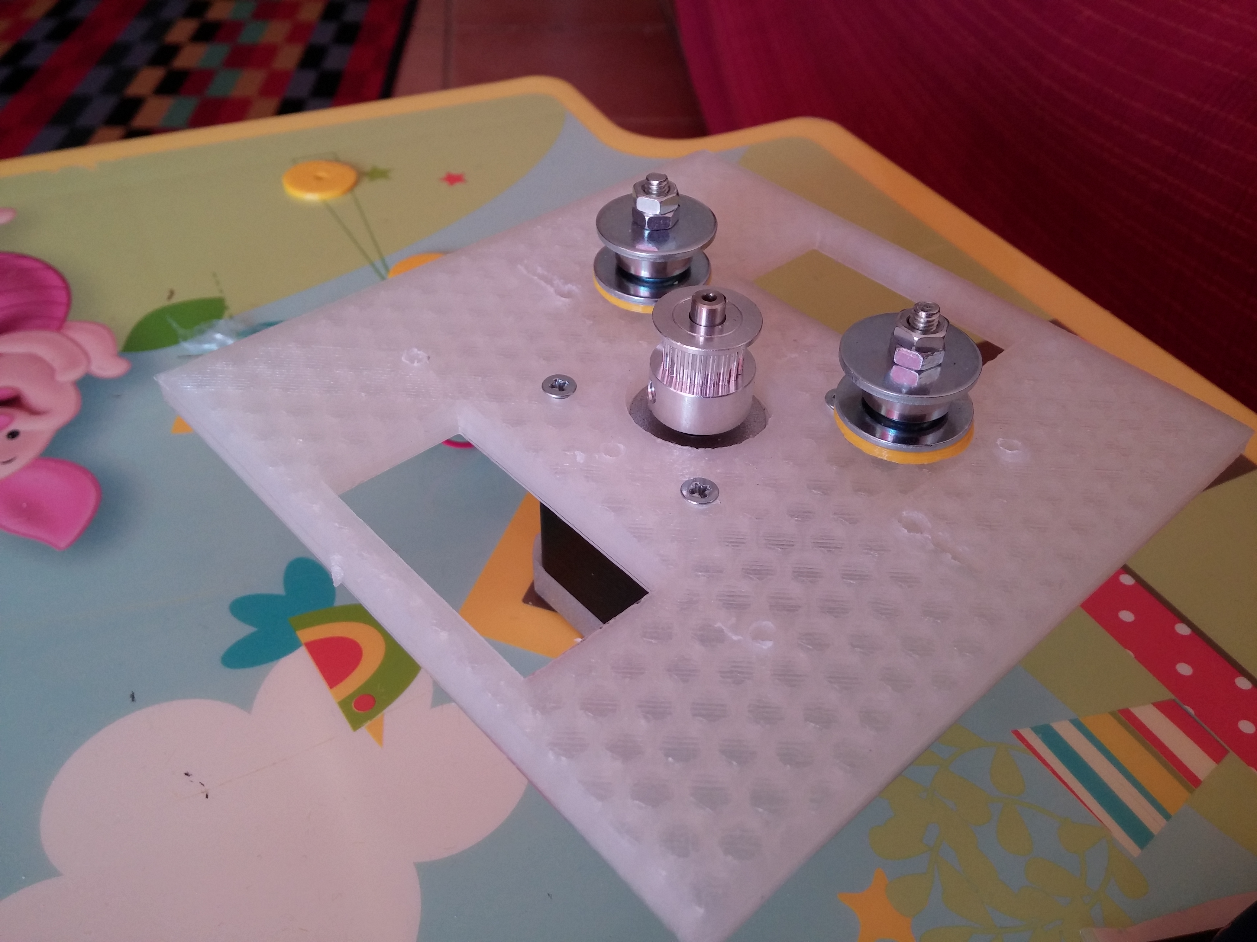
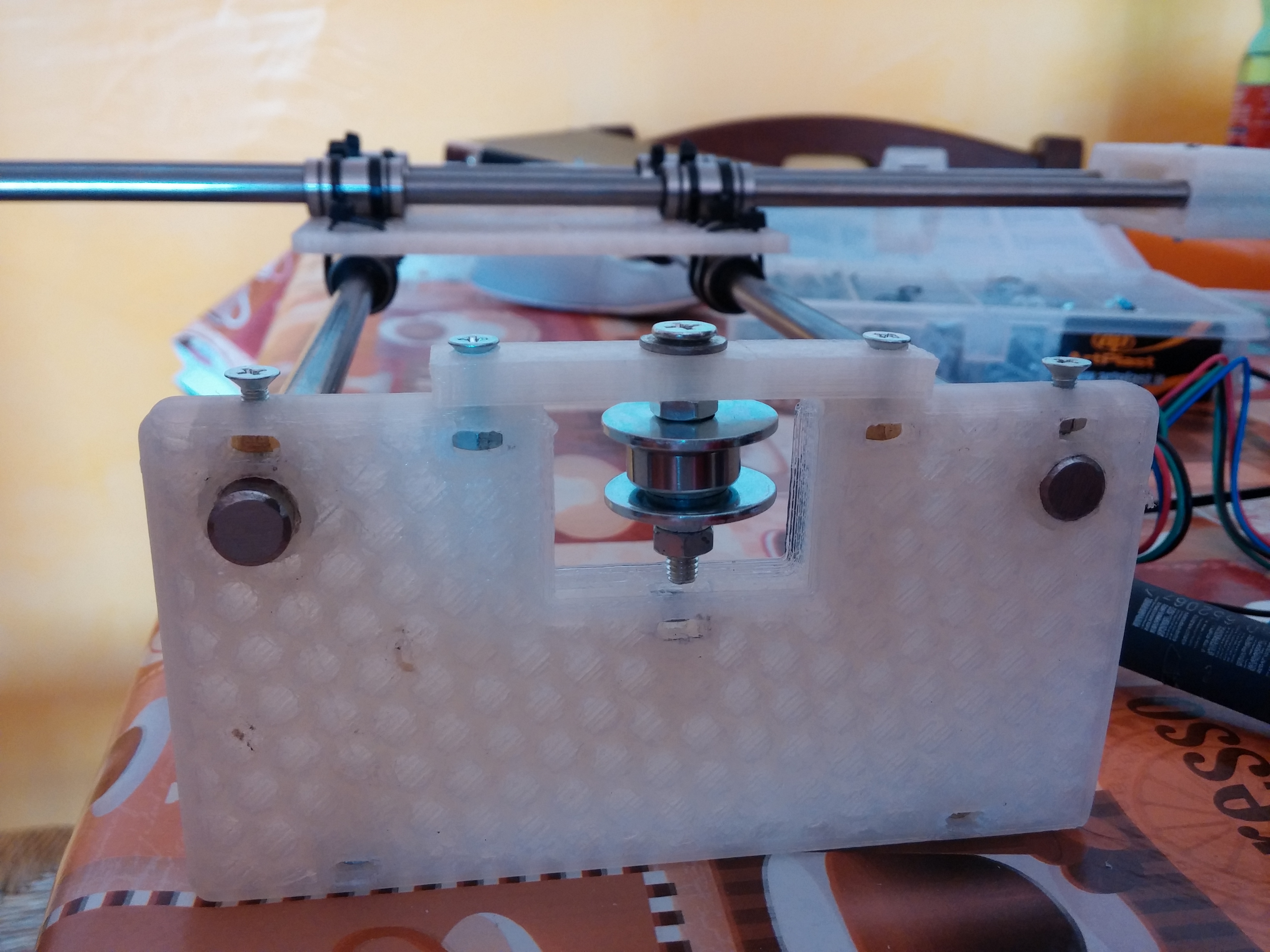


Building

I don’t have a step-by-step building manual, the building is easy if the plastics are well printed. I enclose some pictures that can help to build the plotter.

20150530_174015 20150510_092521 20150510_092510 20150510_092459 20150510_092430 20150510_092359


20096119891_de5feeacb5_o


Software chain

The plotter works starting from an picture or a drawing in order to generate a code (GCODE) that can be put inside the Arduino in order to move correctly the plotter. The process is:


grbl process


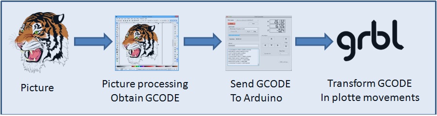
Picture processing to obtain the GCode

I used 3 ways:

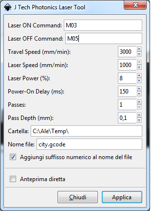
  • Inkscape: this open source program can transform a picture or, better, a SVG picture in GCODE. This is possible thanks to a plug-in: J Tech Photonic Laser Tool. Below an example of the usage. You can use M03 to lower the pen (drawing) and M05 to upper the pen (no drawing). Put a value on the field Power-On-Delay (i.e. 150ms) because the servo needs a  little time to perform the movement. For the Laser power (%) field see the GRBL section of this tutorial

JT photonics laser tool


  • Death to Sharpie: This is an amazing sw made by Scott Cooper in Processing that I customized for the plotter. You can see instructions and examples here. You can take the source code customized here.


  • Hatch4_Gcode2: This is a simple code made by me. It uses the opencv in Processing. It starts with a canny edge detection and after performs an hatching in the gray zones of the image. You can take the source code here


Send Gcode to Arduino

There are many sw that can send Gcode to Arduino. I use the GRBL Controller, but you can use what you want


GRBL with Servo management

The amazing GRBL is the core of the plotter inside the Arduino Uno. But GRBL has a little problem. It works only with stepper motors and Cartesio has one servomotor to raise the pen. So I made some changes to GRBL to drive a servo motor. In fact this is a fork of GRBL 0.9i and it is published here.

See github to understand how you can change the parameters if you want to customize it.

I post also the GRBL configuration I use for the plotter here.


I hope you have fun building the Cartesio plotter.


Processing and Opencv 2.3.1 – Contours detection and polynomial approximation

In the last episode of this short introduction to Opencv and Processing I want to show an algorithm that allows  to appreciate how with the libraries JavaCvPro you can use the OpenCV to implement an algorithm more sophisticated than the basic ones that I have proposed till now.

In this example I make the image edge detection. Then the contours detection is obtained and hence the contours are approximated by polynomial curve. In particular, the polynomial is a set of points that can be represented for example with the segments.
The code is organized as a function java but it is simple to adapt for different uses.


// -- opencv linearization variables
int iterazione=0;
int cc=-1;
int [][] E;
// ********************************************************
// OpenCV - Processing with JavaCvPro
// Edge detection - contour detection - polynomial approximation
// ********************************************************
Pimage goFilterCV(PImage draft) {

  E = new int[ow*oh][3]; // matrix for vertex list - weigth * height

  opencv.allocate(ow, oh); //allocate space for image in opencv

  //-- copy draft image to opencv IplImage with javacvpro library
  opencv_core.IplImage opencvImgSrc=opencv.fromPImage(draft);  // copy draft --> IplImage
  opencv_core.CvSize mySize=opencvImgSrc.cvSize();             // take the size of IplImage

  opencv_core.IplImage opencvImgDest= opencv_core.cvCreateImage(mySize, opencv_core.IPL_DEPTH_8U, 3); // build an image IplImage , 3 channels

  //--- bilateral filter effect
  for (int i=0; i<10; i++) {
    opencv_imgproc.bilateralFilter(opencvImgSrc, opencvImgDest, 3, 20.0, 50.0, 0 ); // applique un effet Flou gaussien 
    opencv_core.cvCopy(opencvImgDest, opencvImgSrc);
  }
  filter1 = createImage(ow,oh,RGB);
  filter1=toPImage(opencvImgDest);

  //-- define IplImage
  opencv_core.IplImage iplImgGray;
  opencv_core.IplImage iplImgGray1;
  iplImgGray = opencv_core.cvCreateImage(mySize, opencv_core.IPL_DEPTH_8U, 1);   // build an image IplImage , 1 channels - only gray
  iplImgGray1= opencv_core.cvCreateImage(mySize, opencv_core.IPL_DEPTH_8U, 1);   // build an image IplImage , 1 channels - only gray

  //-- transform colors in gray levels
  opencv_imgproc.cvCvtColor(opencvImgSrc, iplImgGray, opencv_imgproc.CV_RGB2GRAY);

  //-- edge detection - canny algo
  opencv_imgproc.cvCanny(iplImgGray, iplImgGray1, 100.0, 130.0, 3 );
  //opencv_imgproc.cvDilate(iplImgGray1, iplImgGray1, null , 1); // in alternative you can use the dilate function to better find the edges

  //-- contour detection
  opencv_core.CvMemStorage mem = opencv_core.CvMemStorage.create();
  opencv_core.CvSeq contour = new opencv_core.CvSeq(null);
  int total=opencv_imgproc.cvFindContours(iplImgGray1, mem, contour, Loader.sizeof(opencv_core.CvContour.class), opencv_imgproc.CV_RETR_LIST, opencv_imgproc.CV_CHAIN_APPROX_NONE);
  println("total point cvFindContours:"+total);

  //-- polynomial approximation
  while (contour != null && !contour.isNull ()) {
    iterazione++; //number of interactions
    opencv_core.CvSeq poly = null;
    if (contour.elem_size() > 0) {
      poly = opencv_imgproc.cvApproxPoly(contour, Loader.sizeof(opencv_core.CvContour.class), mem, opencv_imgproc.CV_POLY_APPROX_DP, 3, -1);

      //transfer to matrix
      int n = poly.total();
      opencv_core.CvPoint points = new opencv_core.CvPoint(n);
      opencv_core.cvCvtSeqToArray(poly, points.position(0), opencv_core.CV_WHOLE_SEQ);
      for (int i = 0; i < n; i++) {
        cc++;
        opencv_core.CvPoint pt = points.position(i);
        int x = pt.x();
        int y = pt.y();
        E[cc][0]=x;
        E[cc][1]=y;
        E[cc][2]=iterazione;
        // println("pts:"+i+" x:"+x+" y:"+y);
      }
    }
    contour = contour.h_next();
  } //end polynomial approx

 // -- print some values for debugging purposes
 // for (int i = 0; i < 100; i++) //contatore to have all the points
 // println(E[i][0]+" "+E[i][1]+" "+E[i][2]);

  draft=toPImage(iplImgGray1); // return draft - PImage
  return (draft);

}

// ********************************************************
// take an IplImage and give a PImage
// ********************************************************
PImage toPImage (opencv_core.IplImage iplImgIn) { // take an IplImage and give a PImage
  //--- put the IplImage in a bufferedImage
  BufferedImage bufImg=iplImgIn.getBufferedImage(); 

  //---- build a PImage with the same size of IplImage--- 
  PImage imgOut = createImage(iplImgIn.width(), iplImgIn.height(), RGB);

  // put the pixel of IplImage to imgOut.pixels of PImage
  bufImg.getRGB(0, 0, iplImgIn.width(), iplImgIn.height(), imgOut.pixels, 0, iplImgIn.width()); 

  imgOut.updatePixels(); // PImage update

  return(imgOut); // return the PImage
}

Processing and Opencv 2.3.1 – Using JavaCvPro

To use the OpenCV 2.3.1 in Processing  the shortest and easiest way is to use the JavaCvPro by X.Hinault.
The library JavaCVPro allows to use the OpenCV primitives in a very simple and immediate.
To use the webcam, it requires the library GSVideo  that can be installed in Processing / modes / java / libraries (for Processing 1.5).

Here’s an example of JavaCVPro usage:

// Programme d'exemple de la librairie javacvPro
// par X. HINAULT - octobre 2011
// Tous droits réservés - Licence GPLv3

// Exemple fonction contrast()

import monclubelec.javacvPro.*; // importe la librairie javacvPro

PImage img;

String url="http://www.mon-club-elec.fr/mes_images/online/lena.jpg"; // String contenant l'adresse internet de l'image à utiliser

OpenCV opencv; // déclare un objet OpenCV principal

void setup(){ // fonction d'initialisation exécutée 1 fois au démarrage

        //-- charge image utilisée --- 
        img=loadImage(url,"jpg"); // crée un PImage contenant le fichier à partir adresse web

        //--- initialise OpenCV ---
        opencv = new OpenCV(this); // initialise objet OpenCV à partir du parent This
        opencv.allocate(img.width, img.height); // initialise les buffers OpenCv à la taille de l'image

        opencv.copy(img); // charge le PImage dans le buffer OpenCV

        //--- initialise fenêtre Processing 
        size (opencv.width()*2, opencv.height()); // crée une fenêtre Processing de la 2xtaille du buffer principal OpenCV
        //size (img.width, img.height); // aalternative en se basant sur l'image d'origine

        //--- affiche image de départ --- 
        image(opencv.getBuffer(),0,0); // affiche le buffer principal OpenCV dans la fenêtre Processing

        //--- opérations sur image ---
        opencv.contrast(+50); // applique réglage contraste sur le buffer principal OpenCV

        //--- affiche image finale --- 
        image(opencv.getBuffer(),opencv.width(),0); // affiche le buffer principal OpenCV dans la fenêtre Processing

       noLoop(); // stop programme 
}

void  draw() { // fonction exécutée en boucle

}


The code is very simple. All the opencv instructions are called simply using ‘opencv.’ before the real instruction. You can use the opencv instructions translated in Processing by X. Hinault in the JavaCvPro libraries.

But it is very interesting to mix OpenCv instruction supported by JavaCvPro libraries and native OpenCv instructions. The JavaCvPro allow to use also the native OpenCV instruction. This is a powerful tool!!!

In the example below, only native
OpenCV instructions are used.

// Example of using native OpenCVPro instruction in Processing
// Robottini.altervista.org
// example by X.Hinault modified
// Licence GPLv3

// Bilinear filter example

import com.googlecode.javacv.*;
import com.googlecode.javacv.cpp.*;
import monclubelec.javacvPro.*;
import java.awt.image.BufferedImage;
PImage imgDest, OrigImg;
void setup() {
  size(640, 240);
  String cheminFichier="C:/Users/Nane/Dropbox/Sorgenti Arduino/Jarkman/Foto/gioconda1.jpg";; 
  OrigImg=loadImage(cheminFichier,"jpg"); 
  //---- appel direct des fonctions de la librairie javacv ---- 
  //--- chargement d'un fichier image 
  opencv_core.IplImage opencvImgSrc= opencv_highgui.cvLoadImage(cheminFichier);

  opencv_core.CvSize mySize=opencvImgSrc.cvSize(); // récupère la taille de l'image 

  opencv_core.IplImage opencvImgDest= opencv_core.cvCreateImage(mySize, opencv_core.IPL_DEPTH_8U, 3); // crée une image IplImage , 3 canaux

  //--- application d'effet opencv ---
 for (int i=0; i<20; i++)
    opencv_imgproc.bilateralFilter(opencvImgSrc, opencvImgDest, 3,120.0, 190.00,1 ); // applique un effet Flou gaussien 

//============ récupérer une image openCV dans Processing ===== 
  //--- récupérer l'objet IplImage dans un BufferedImage 
  BufferedImage bufImg=opencvImgDest.getBufferedImage(); // récupère l'image

  //---- créer un PImage --- 
  PImage img = createImage(320,240, PConstants.RGB); 

  // charge les pixels de l'image buffer dans img.pixels
  bufImg.getRGB(0, 0, 320, 240, img.pixels, 0, 320); 
  img.updatePixels();
  image(OrigImg,0,0); 
  image(img,320,0); // affiche l'image
}
void draw() {

}


In this case the OpenCv instructions for Processing are used only in the last part of the code, in order to show the images. The coding of the native OpenCV instructions is more difficult, but very very powerful. It is possible to use almost the whole set of instructions offered by the OpenCv 2.3.1.