Archive for category Tips

Kalman filter vs Complementary filter

Note: At the bottom of the post the complete source code

The use of accelerometer and gyroscope to build little robots, such as the self-balancing, requires a math filter in order to merge the signals returned by the sensors.
The gyroscope has a drift and in a few time the values returned are completely wrong. The accelerometer, from the other side,  returns a true value when the acceleration is progressive but it suffers much the vibrations, returning values of the angle wrong.

Usually a math filter is used to mix and merge the two values, in order to have a correct value: the  Kalman filter . This is the best filter you can use, even from a theoretical point of view, since it is one that minimizes the errors from the true signal value. However it is very difficult (see here) to understand.  In fact, the filter needs to be able to calculate the coefficients of the matrices, the process-based error, measurement error, etc. that are not trivial.

In the hobbistic world, recently are emerging other filters, called complementary filters. In fact, they manage both high-pass and low-pass filters simultaneously. The low pass filter filters high frequency signals (such as the accelerometer in the case of vibration) and low pass filters that filter low frequency signals (such as the drift of the gyroscope). By combining these filters, you get a good signal, without the complications of the Kalman filter.

Making a study from a theoretical point of view, the discussion is complicated and is beyond the scope of this tutorial. The complementary filters can be have different ‘orders’. Here I speak about the so-called first-order filter that filter already well, and the second-order filter which filter even better. Clearly, going from first to second order, the algorithm is more complicated to use and perhaps there is no gain so obvious  to justify the increase in complexity.
A great introduction to the first order complementary filters applied to the an accelerometer and a gyroscope, comes from MIT (here). It introduces the filter in a a very simple  mode. On this document is based the first Arduino algorithm:

// a=tau / (tau + loop time)
// newAngle = angle measured with atan2 using the accelerometer
// newRate = angle measured using the gyro
// looptime = loop time in millis()

float tau=0.075;
float a=0.0;

float Complementary(float newAngle, float newRate,int looptime) {
float dtC = float(looptime)/1000.0;
a=tau/(tau+dtC);
x_angleC= a* (x_angleC + newRate * dtC) + (1-a) * (newAngle);
return x_angleC;
}

It ‘enough to choose the response time of tau, to send the arguments, ie the angle measured with the accelerometer and the gyroscope, the time of the loop and you get in two lines, the angle calculated by the filter.

The algorithm at the base of the second order complementary filter is described here. Indeed it is not described at all, but now we’ve figured out how the filter works by the MIT’s documentation. The principle is the same, the algorithm is more complicated. The translation of this algorithm for the Arduino:

// newAngle = angle measured with atan2 using the accelerometer
// newRate = angle measured using the gyro
// looptime = loop time in millis()

float Complementary2(float newAngle, float newRate,int looptime) {
float k=10;
float dtc2=float(looptime)/1000.0;

x1 = (newAngle -   x_angle2C)*k*k;
y1 = dtc2*x1 + y1;
x2 = y1 + (newAngle -   x_angle2C)*2*k + newRate;
x_angle2C = dtc2*x2 + x_angle2C;

return x_angle2C;
}

Here too we just have  to set the k and magically we get the angle.

If we want to apply the Kalman filter, we can re-use one of the codes already present in internet. This is the code that I copied from the Arduino forum (here):


// KasBot V1 - Kalman filter module

float Q_angle  =  0.01; //0.001
float Q_gyro   =  0.0003;  //0.003
float R_angle  =  0.01;  //0.03

float x_bias = 0;
float P_00 = 0, P_01 = 0, P_10 = 0, P_11 = 0;
float  y, S;
float K_0, K_1;

// newAngle = angle measured with atan2 using the accelerometer
// newRate = angle measured using the gyro
// looptime = loop time in millis()

float kalmanCalculate(float newAngle, float newRate,int looptime)
{
float dt = float(looptime)/1000;
x_angle += dt * (newRate - x_bias);
P_00 +=  - dt * (P_10 + P_01) + Q_angle * dt;
P_01 +=  - dt * P_11;
P_10 +=  - dt * P_11;
P_11 +=  + Q_gyro * dt;

y = newAngle - x_angle;
S = P_00 + R_angle;
K_0 = P_00 / S;
K_1 = P_10 / S;

x_angle +=  K_0 * y;
x_bias  +=  K_1 * y;
P_00 -= K_0 * P_00;
P_01 -= K_0 * P_01;
P_10 -= K_1 * P_00;
P_11 -= K_1 * P_01;

return x_angle;
}

To get the answer, you have to set 3 parameters: Q_angle, R_angle,R_gyro. The activity is a bit complicated .
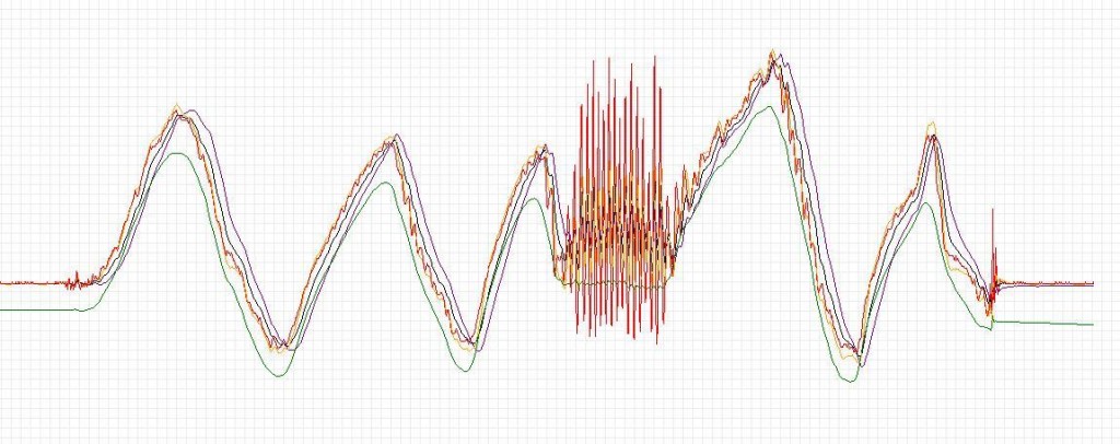
But what happens with these algorithms?  Similar curves are obtained?  Here’s a comparison:
There are 5 curves:

Color lines:

  • Red – accelerometer
  • Green – Gyro
  • Blue – Kalman filter
  • Black – complementary filter
  • Yellow – the second order complementary filter

As you can see the signals filtered are very similarly. Note that in the presence of vibrations, the accelerometer (red) generally go crazy.  The gyro (green) has a very strong drift increasing int the time.

Now let’s see a comparison only between a filtered signal. That kalman (green), complementary (black) and complementary second-order (yellow). You can see how the Kalman is a bit late vs complementary filters, but it is more responsive to the vibration. In this case the second order filter does not return an ideal curve, probably I have to work a bit on the coefficients.
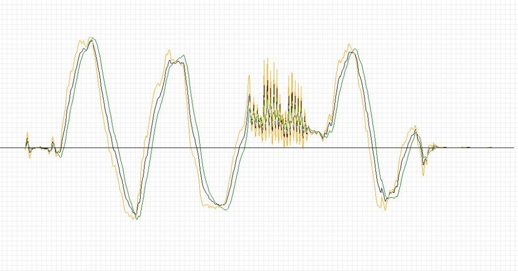
In conclusion I think that the complementary filter, in this case the first order, can be used in place of the Kalman filter. The smoothing is good and the algorithm is much simpler than Kalman.

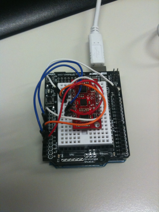
The hardware I used was composed of:
– Arduino 2009
– 6-axis IMU SparkFun Razor 6 DOF
This is the complete source code: Filters1

Tags: ,

12 servos controller low cost

 Building a robot with wheels or with legs needs a design completly different. One of the biggest difference is the type and number of motors.

While for a robot with wheels usually 2 or 4 servos or gear motors are enough, when we speak about a robot with legs, the number of motors increases dramatically. It is not uncommon to see a hexapod robot with 18 servos.
A quadrapod robot has usually 8 or 12 servos, depending on the number of joints. Luckily, compared to robot with wheels, usually are not required servomotors with continuous rotation or gearmotors. Standard servos (0-180 degrees) are enough.
Servomotors are driven with PWM and Arduino 2009 or Arduino Uno have 6 PWM pin. And this is a problem. And if you want to use also other sensors using digital pins, the situation is not good, because the Arduino’s digital pins are only 14, and 2 of wich are used for the serial port communication (pin 0 and 1).
It is possible to use the Arduino Mega, with 14 PWM pin, but it is very expensive (50 euros and more).
Searching in internet, I found a low cost chip, using I2C protocol that can drive 12 servos. First good news, the I2C protocol uses only the analog pins 4 and 5. Second good news is that you can use up to 8 chip, so it is possible to drive up to 8×12=96 servos with only 2 analog pins, the 4 and 5. Third good news is that the chip costs about 4 euros and half. A price that can be accepted by every robot builder.
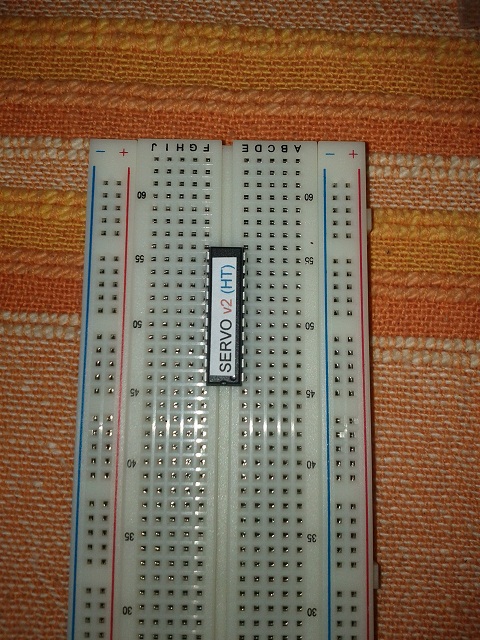
This is the magic chip:


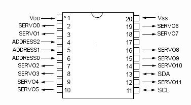
It is a DIP chip with 20 pins.The chip is made by Hobbytronics (here).  This is the pins schema:


This is the pins usage:

VDD = +5 V
Vss = GND
SDA, SLC are pins I2C that are connected to Arduino’s pins 4 and 5 and also connected to the Arduino +5 V using the pull-up resistors. The value is between 1K and 10K Ohm (I used the 3.3k Ohm).
Address1, 2, 3 are the pins that you can use to change the I2C address of the chip(usually not needed, unless you uses more than one chip, in this case it is necessary to differentiate the addresses).
SERVO01 … SERVO11 are pins connected  to the control pin of the servos (the others are connected to +5 V and GND).
I did a test  and I think it works fine.
Here is a short video I made:


This is the datasheet.

This is the code used in the video.

Below my code:

// I2C servo controller by www.hobbytronics.co.uk
// written by Alegiaco - July 2011

#include <Wire.h>

const int  servoslave_address=40;   // I2C Address of ADC Chip 
int gradServo[12];

void setup()
{

servo12Setup();

}

void loop()
{
moveServo(5,0); // move servo 5 to 0 degrees
delay(1000);
moveServo(5,90); //move servo 5 to 90 degrees
delay(1000);
moveServo(5,180);  //move servo 5 to 180 degrees
delay(1000);

// move servo 4 and 5 to 100 degrees
gradServo[4]=100;
gradServo[5]=100;
moveServoSet(4,5,gradServo);
delay(1000);

// move servo 4 and 5 to 180 degrees
gradServo[4]=180;
gradServo[5]=180;
moveServoSet(4,5,gradServo);

delay(1000);
}

void servo12Setup(){
 Wire.begin();              // join i2c bus (address optional for master)
  // Optionally set mode to standard 
  // – comment out this section if extended mode required
  Wire.beginTransmission(servoslave_address); // transmit to device
  Wire.send(20);             // servo register address 20
  Wire.send(1);              // 1 = extended mode (0-180 degrees)
  Wire.endTransmission();    // stop transmitting 
  delay(1);
}

void moveServo(int numServo, int deg) {
    Wire.beginTransmission(servoslave_address); // transmit to device
    Wire.send(numServo);               // servo register to start from
    Serial.println(numServo);
    float degre=((deg/180.0)*255.0);    // transform in format compatible with servo controller
    int degree=int(degre);
    Wire.send(degree);           // send 12 bytes of data
    Wire.endTransmission();    // stop transmitting 
    delay(1);                  // waits
  } 

void moveServoSet(int numServoStart, int numServoEnd, int valServo[12]) {
    Wire.beginTransmission(servoslave_address); // transmit to device
    Wire.send(numServoStart);               // servo register to start from
    for (int j=numServoStart;j<=numServoEnd;j++) {
      float degre=valServo[j]/180.0*255.0;
      int degree=int(degre);
      Wire.send(degree);           // send 12 bytes of data
      }
    Wire.endTransmission();    // stop transmitting 
    delay(1);                  // waits 

    }

Tags:

Arduino and real time charts in Excel

One of the most important things in the robot design is the possibility to check and control the values feeded by the analogic sensors, i.e. accelerometers, gyros, IR sensors.
In order to view the sensor values you can use the Serial Port that can be displayed in the Serial Monitor inside the Arduino IDE environment.
But it isn’t possible to show charts or save the data read from the sensors.
There are several software that allow to show the graphs derived from the sensors data, and I published in the past a tutorial (here).
Usually you use Processing or similar language that require always to write some code. You have to write code to change the charts or to implement new lines in the graphs.
I thought that the ideal situation would be to use a software that everyone knows: Microsoft Excel.

If it were possible to use Excel to receive the data from the serial port, it would be easy to make very nice and user friendly charts.
I searched in Google and i found a sw that allows easily to view the serial port values in Excel.
The sw is made by a competitor of Arduino, Parallax, the company that sells the Boe-Bot and the Propeller, wich are in direct competition with Arduino.

The sw is called PLX-DAQ and it is a free software. You can download it here. It works only in Windows, sorry.
In practice it is a little sw in VBA that adds some features to Excel to receive and elaborate real time data. If the data are in Excel it is also possible to save them in a file and it is possible to use the amazing function library already present in the spreadsheet software. The documentation about PLX-DAQ is complete and clear.

The PLX-DAQ takes commands in uppercase and every data row have to end with a ‘carriage return’. The serial port speed required by PLX-DAQ is particular, because it derives from Parallax world. In any case the rate is from 9600 bit/sec to 128.000 bit/sec. The speed of 128.000 bit/sec works fine in the Arduino!!

The main commands are:

  • LABEL used to define the column headings. The command format is:  Serial.println (“LABEL, INT_COLUMN”);
  • DATE, TIME that allows the serial port to send data to Excel. The first field is always TIME, then the fields of interest (val). The command format is:  Serial. print (“DATE, TIME,”);  Serial.println (val)
  • ROW, SET, k,  allows you to define the next line to write. It is useful if you want to plot n data and then go back to first row and cycle. For example, you can plot 1000 data on the chart and then start again from the first position, in order to avoid a graph too large. The command format is: Serial.println (ROW, SET, 2) put the cursor in the second line next step.

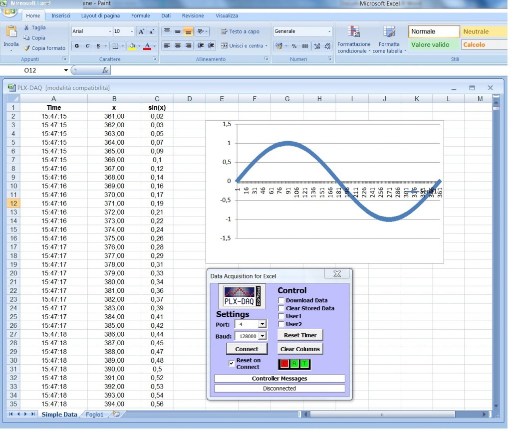
Here’s an example that shows Excel function sin (x).

The Arduino code:


int x = 0;
int row = 0;
void setup() {
  Serial.begin(128000); // opens serial port, sets data rate to 128000 bps
  Serial.println("CLEARDATA");
  Serial.println("LABEL,Time,x,sin(x)");
}

void loop() {
  Serial.print("DATA,TIME,"); Serial.print(x); Serial.print(","); Serial.println(sin(x*PI/180));
  row++;
  x++;
  if (row > 360) 
   {
    row=0;
    Serial.println("ROW,SET,2");
   }
  delay(100);
}


PLX-DAQ enable a more complex interaction with Excel. It can take the cell values from Excel, it can read and write check box. You can see the PLX-DAW documentation for other details.

Tags: , ,