Delta robot with Arduino

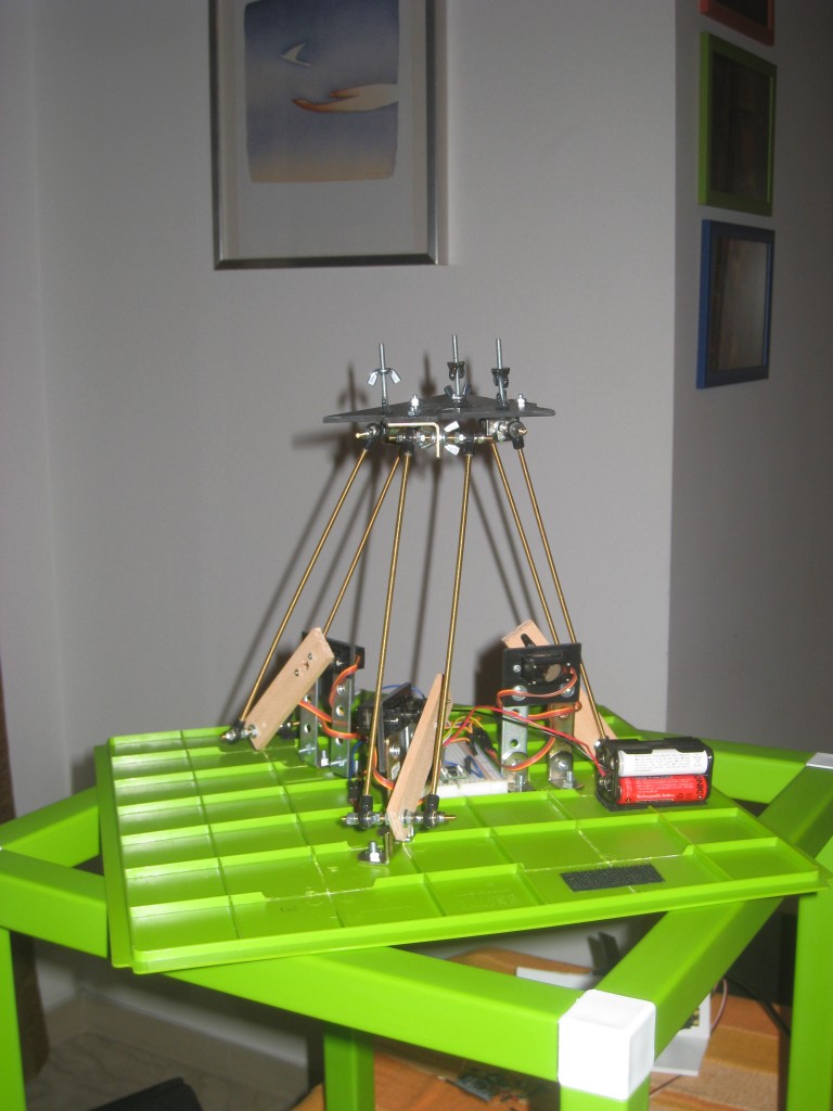
Today I present my first Delta robot made with Arduino. The Delta robot structure was designed by a professor at the Technical University of Lausanne in 1985.  It is a parallel robot, and within two decades has become the star of pick and place industrial robots . The delta robot distinctive elements are two:

  • The robot geometry which simplifies the equations of motion (kinematics)
  • The great idea to anchor the robot upside down so that it has the motors connected to the base. This is very important because while the robot works, the motors remain attached at the base, allowing the robot to have arms very light. Lightness means low friction, low inertia, low power motors, precision, speed, fast acceleration and deceleration.

These are two examples of delta robot:


These aren’t laboratory prototypes, but commercial robots and they cost about 50-60.000 euros. I tried to build a simple delta robot with Arduino. My Delta robot works like the commercial Delta robot, ie, in inverse kinematics. Given a point x, y, z in space, in real time Arduino calculates the angles of the servomotors that allow  to reach that point in space.

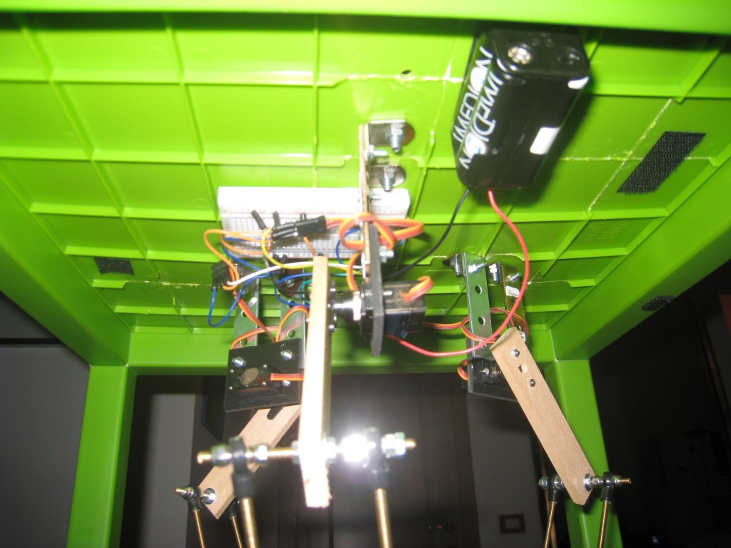
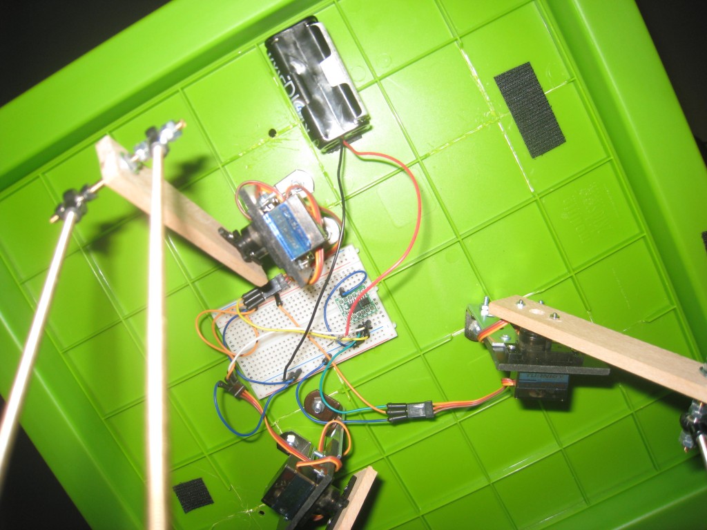
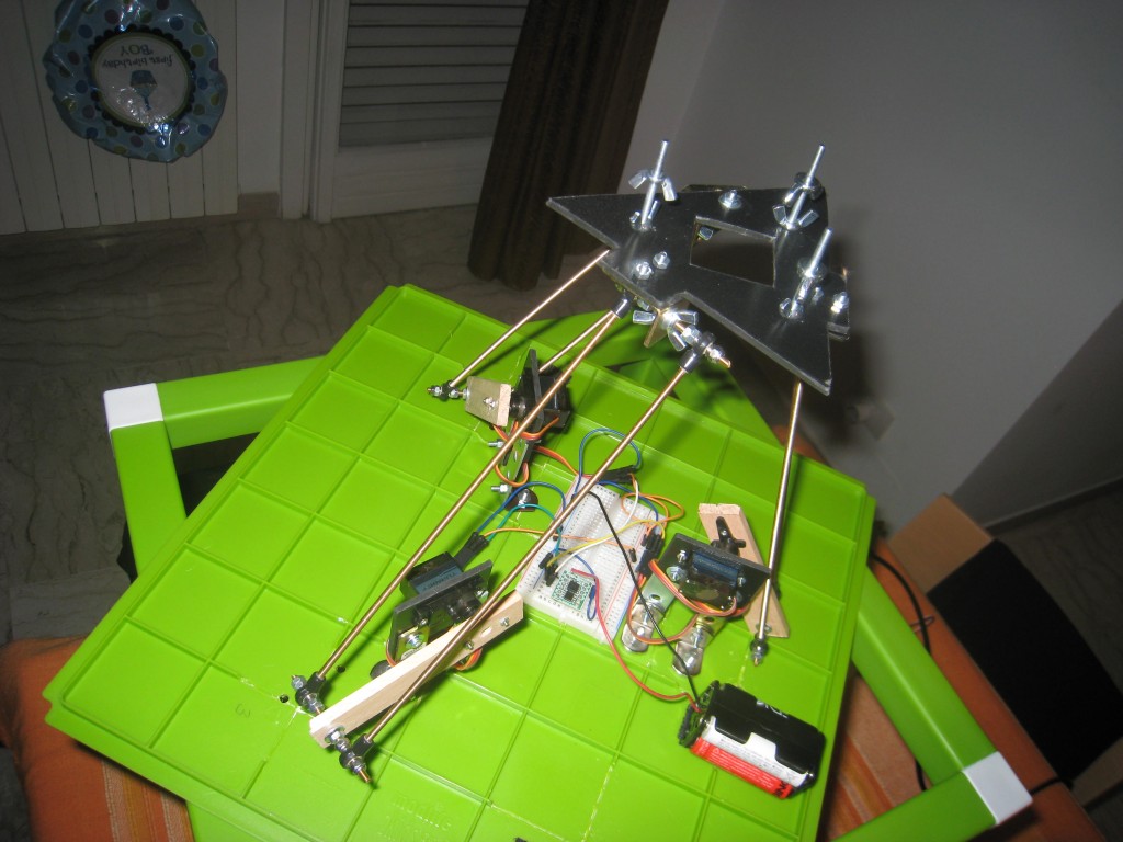
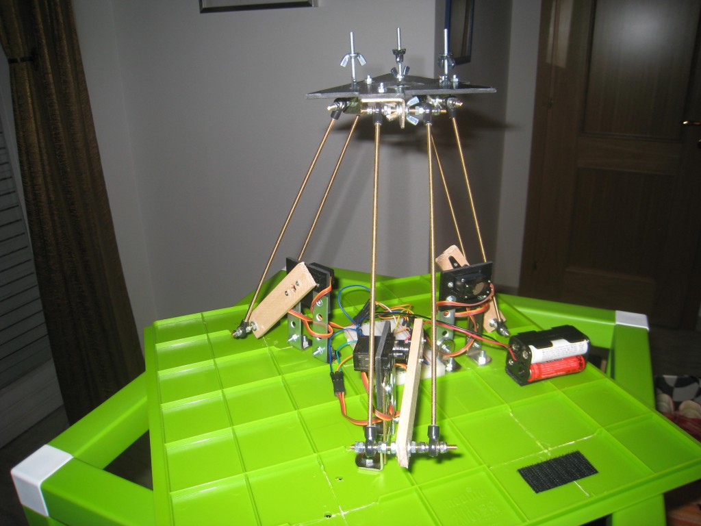
The Delta robot has two triangular plates. A higher which is fixed and the lower is free. The servo motors are fixed to the top plate. The gripping tool (i.e. an electromagnet, a gripper, a vacuum suction cup), is fixed to the lower plate. The two plates are triangular equilateral, that is, equal sides and equal angles of 60 °.

The Delta  has 3 servo motors and two arms for each servo. One is integral with the servo. The other arm is free to rotate in all directions and it is connected to the lower small triangle. In order to ensure the free turning, the second arm is linked with ball joints. To find the ball joints has not been easy. I found something about the steering of the machine model. Just search on google “joint Uniball” and you can find little cheap joints.

A very good explanation about the the Delta robot geometry and a very effective explanation of inverse and direct kinematics formulas can be found here . You can find also the code that calculates the inverse kinematic.

These are some Delta robot pictures (with an ATtiny85 microcontroller).


The end effector can be used with different tools. I tried a vacuum syringe and  a drawing pen.

These below are some videos with different tools.


The first experiment with a simple trajectory (a circle).


The Delta robot drove by a mouse with Processing. The code is available here.


The Delta robot in  pick and place configuration. The code is available here.


The Delta robot drawing. This is a first draft. The code is available here.
 

Tags: , ,

Auduino

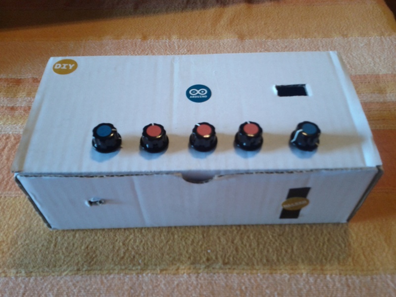
I have two friends that play “industrial music” (link).  It is a sort of mix between noises and sounds, very interesting. You can like it or not, but anyway it is interesting. They saw in the Wired magazine, the istructions to realize an Auduino. It is a synthetizer made with an Arduino and some potentiometers. It is very simple to realize. They asked me if I could make this Arduino, because they are always searching for new instruments, new sounds, new noises.

The link to Auduino explanation: http://code.google.com/p/tinkerit/wiki/Auduino

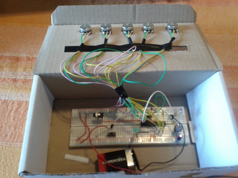
So I realized an Auduino. Because to use an Arduino Uno for a stand-alone application is not a wise decision, I built an Arduino in a breadboard, using these instructions (link)

I modified a little the schema to be more simple. This is the result:


This is Auduino in action:


Tags:

Kalman filter vs Complementary filter

Note: At the bottom of the post the complete source code

The use of accelerometer and gyroscope to build little robots, such as the self-balancing, requires a math filter in order to merge the signals returned by the sensors.
The gyroscope has a drift and in a few time the values returned are completely wrong. The accelerometer, from the other side,  returns a true value when the acceleration is progressive but it suffers much the vibrations, returning values of the angle wrong.

Usually a math filter is used to mix and merge the two values, in order to have a correct value: the  Kalman filter . This is the best filter you can use, even from a theoretical point of view, since it is one that minimizes the errors from the true signal value. However it is very difficult (see here) to understand.  In fact, the filter needs to be able to calculate the coefficients of the matrices, the process-based error, measurement error, etc. that are not trivial.

In the hobbistic world, recently are emerging other filters, called complementary filters. In fact, they manage both high-pass and low-pass filters simultaneously. The low pass filter filters high frequency signals (such as the accelerometer in the case of vibration) and low pass filters that filter low frequency signals (such as the drift of the gyroscope). By combining these filters, you get a good signal, without the complications of the Kalman filter.

Making a study from a theoretical point of view, the discussion is complicated and is beyond the scope of this tutorial. The complementary filters can be have different ‘orders’. Here I speak about the so-called first-order filter that filter already well, and the second-order filter which filter even better. Clearly, going from first to second order, the algorithm is more complicated to use and perhaps there is no gain so obvious  to justify the increase in complexity.
A great introduction to the first order complementary filters applied to the an accelerometer and a gyroscope, comes from MIT (here). It introduces the filter in a a very simple  mode. On this document is based the first Arduino algorithm:

// a=tau / (tau + loop time)
// newAngle = angle measured with atan2 using the accelerometer
// newRate = angle measured using the gyro
// looptime = loop time in millis()

float tau=0.075;
float a=0.0;

float Complementary(float newAngle, float newRate,int looptime) {
float dtC = float(looptime)/1000.0;
a=tau/(tau+dtC);
x_angleC= a* (x_angleC + newRate * dtC) + (1-a) * (newAngle);
return x_angleC;
}

It ‘enough to choose the response time of tau, to send the arguments, ie the angle measured with the accelerometer and the gyroscope, the time of the loop and you get in two lines, the angle calculated by the filter.

The algorithm at the base of the second order complementary filter is described here. Indeed it is not described at all, but now we’ve figured out how the filter works by the MIT’s documentation. The principle is the same, the algorithm is more complicated. The translation of this algorithm for the Arduino:

// newAngle = angle measured with atan2 using the accelerometer
// newRate = angle measured using the gyro
// looptime = loop time in millis()

float Complementary2(float newAngle, float newRate,int looptime) {
float k=10;
float dtc2=float(looptime)/1000.0;

x1 = (newAngle -   x_angle2C)*k*k;
y1 = dtc2*x1 + y1;
x2 = y1 + (newAngle -   x_angle2C)*2*k + newRate;
x_angle2C = dtc2*x2 + x_angle2C;

return x_angle2C;
}

Here too we just have  to set the k and magically we get the angle.

If we want to apply the Kalman filter, we can re-use one of the codes already present in internet. This is the code that I copied from the Arduino forum (here):


// KasBot V1 - Kalman filter module

float Q_angle  =  0.01; //0.001
float Q_gyro   =  0.0003;  //0.003
float R_angle  =  0.01;  //0.03

float x_bias = 0;
float P_00 = 0, P_01 = 0, P_10 = 0, P_11 = 0;
float  y, S;
float K_0, K_1;

// newAngle = angle measured with atan2 using the accelerometer
// newRate = angle measured using the gyro
// looptime = loop time in millis()

float kalmanCalculate(float newAngle, float newRate,int looptime)
{
float dt = float(looptime)/1000;
x_angle += dt * (newRate - x_bias);
P_00 +=  - dt * (P_10 + P_01) + Q_angle * dt;
P_01 +=  - dt * P_11;
P_10 +=  - dt * P_11;
P_11 +=  + Q_gyro * dt;

y = newAngle - x_angle;
S = P_00 + R_angle;
K_0 = P_00 / S;
K_1 = P_10 / S;

x_angle +=  K_0 * y;
x_bias  +=  K_1 * y;
P_00 -= K_0 * P_00;
P_01 -= K_0 * P_01;
P_10 -= K_1 * P_00;
P_11 -= K_1 * P_01;

return x_angle;
}

To get the answer, you have to set 3 parameters: Q_angle, R_angle,R_gyro. The activity is a bit complicated .
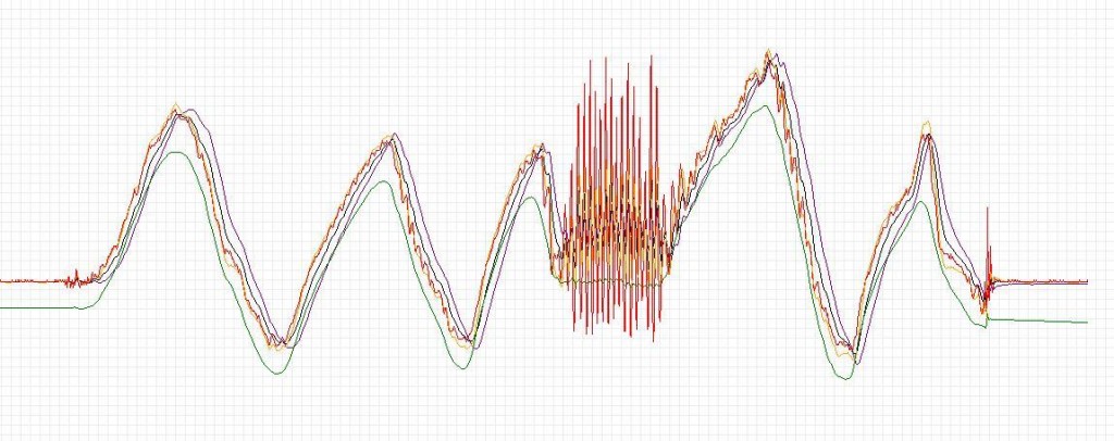
But what happens with these algorithms?  Similar curves are obtained?  Here’s a comparison:
There are 5 curves:

Color lines:

  • Red – accelerometer
  • Green – Gyro
  • Blue – Kalman filter
  • Black – complementary filter
  • Yellow – the second order complementary filter

As you can see the signals filtered are very similarly. Note that in the presence of vibrations, the accelerometer (red) generally go crazy.  The gyro (green) has a very strong drift increasing int the time.

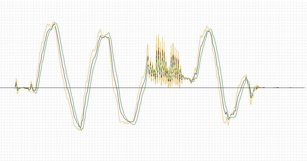
Now let’s see a comparison only between a filtered signal. That kalman (green), complementary (black) and complementary second-order (yellow). You can see how the Kalman is a bit late vs complementary filters, but it is more responsive to the vibration. In this case the second order filter does not return an ideal curve, probably I have to work a bit on the coefficients.

In conclusion I think that the complementary filter, in this case the first order, can be used in place of the Kalman filter. The smoothing is good and the algorithm is much simpler than Kalman.

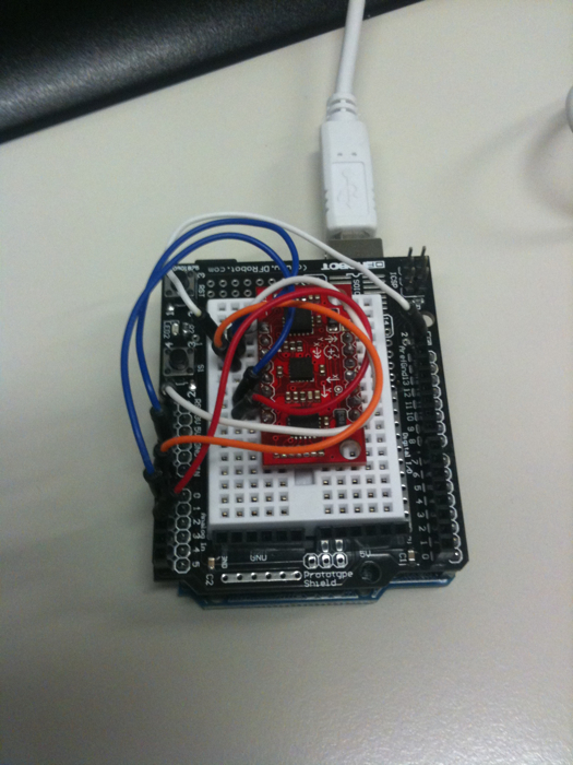
The hardware I used was composed of:
– Arduino 2009
– 6-axis IMU SparkFun Razor 6 DOF

This is the complete source code: Filters1

Tags: ,